
Glaciological inverse methods
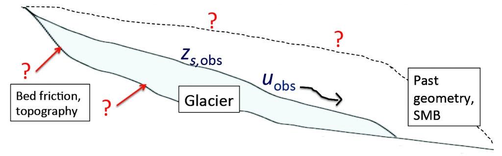
A common theme in glaciology is the need to measure, or estimate, properties that are not accessible – because they are hidden under hundreds of meters of ice, or hidden in the past, and there can be other difficulties besides. Consider the relationship between sliding rate and friction force at the bottom of an ice sheet – the sliding coefficient. It can vary strongly over large expanses – and it strongly determines how sensitive the ice sheet is to changes in climate – and its spatial pattern needed as an input to our ice models. We cannot see everywhere under the ice sheet – and even if we could drill to the bed in a few places, this is not likely to be of value, as there is no apparent relationship between bed properties and sliding coefficient at a given isolated location. Inverse models, however, provide another route. An ice sheet model will use a “guess” for sliding coefficients – and then, depending on how poorly the result matches observations, it will update its guess until a satisfactory match with observations is found. Much of glaciological inverse modelling deals with effective ways to update this guess. I’ve had projects involving inverse modelling at a number of different levels over the years, and I continue to try to improve the way we gather information from glaciological data.
Inverse problems with Higher Order glacier mechanics
The example of sliding coefficients above has a long history in the modelling of ice dynamics. MacAyeal (1992) derived a method to greatly speed up the process of improving the “guess” of the sliding coefficient pattern. Termed a control method, it solves the adjoint of the linearized ice flow model to find the search direction in which model-observation misfit is optimally minimized. By iteration, an optimal solution is reached. In the quarter-century since, this is still the method of choice for glaciological inversions. Most often it is done using a Shallow-Shelf Approximation (SSA) flow model.
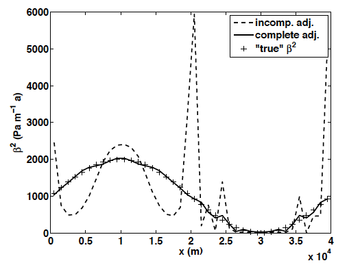
More recently, hybrid models, which retain the ease of solution of the SSA but represent vertical shearing which takes place over a cold bed, which the SSA cannot. The adjoint of a hybrid model was very carefully derived, taking care not to make any approximations (as is usually done for ease of computation). The implications of making such approximations can be seen below in the results of an “identical twin” test, where sliding coefficients are known and model output is treated as data. Using a less accurate adjoint results in a failed recovery of those coefficients.
Relevant publications:
Goldberg 2011
Goldberg and Sergienko 2011
Automatic Differentiation
An adjoint model is essentially the derivative of a model, and, as discussed above, it is enormously helpful in finding the best set of inputs to provide a desired output. There are two general ways to find the adjoint of a numerical model: (1) Starting from the continuous equations, find the adjoint to these equations and discretise, and (2) Discretise the continuous equations into computer code, and then differentiate the computer code, line by line. Historically (1) has been used for ice model inversions. (2) has been applied extensively to ocean models, but its use in ice sheet modelling is limited, which is unfortunate – applying (1) to a time-dependent ice flow model is not an easy feat! On the other hand, (2) is impractical without the aid of Automatic Differentiation (AD) – software which applies the “chain rule” of differentiation at the operation level. Examples of AD tools are TAF, OpenAD, and Tapenade. Still, if care is not taken in writing the code, the AD tools will not work.
AD tools have been applied to an ice-sheet model developed as part of MITgcm, and more recently with the FEniCS software. In a recent study these tools were used to assimilate a decades’ worth of remotely observed data and to assess the susceptibility of a fast flowing ice stream to ocean melt, and they are now being used as part of the International Thwaites Initiative
Relevant publications:
Goldberg and Heimbach 2013
Goldberg et al 2015
Goldberg et al 2016
Goldberg et al 2018
Maddison, Goldberg and Goddard 2019