Ice Sheet-Ocean Interactions

The manner in which ice sheets and ocean interact plays an important role in the global climate. In Antarctica, this interaction is primarily through enormous floating extensions of the ice sheet called ice shelves. The ocean circulates underneath the ice shelves leading to melting and freezing. From the ocean side, this melting and freezing changes the properties of sea water, which can ultimately have impacts on the ocean’s large-scale overturning circulation.

On the ice side, the effect of melting is to thin the ice shelves. While this does not immediately contribute to sea level, it affects the buttressing capacity of the ice shelf – its ability to hold back flow of ice from the continent into the sea. Since the mid-1990s, it is known that the ice shelves of the Amundsen Embayment of West Antarctica have been melting at high rates due to the presence of Circumpolar Deep Water (CDW). It is feared that the speed up of the ice, and the subsequent retreat of grounding lines in the Amundsen, will lead to a positive feedback loop often called Marine Instability – and that sea levels will rise much faster than they do currently in the coming centuries.

Here are some helpful links explaining the above concepts:

Ice-shelf buttressing.

Marine Instability

Circumpolar Deep Water

Here are a few projects I have been or am currently involved with:

Ice-Ocean Coupling

Asynchronous coupling

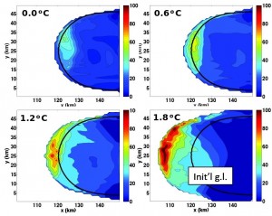
Coupling between land ice and ocean models is important as both land ice and sub-shelf circulation are known to influence each other. We coupled the isopycnal model GOLD to an ice-sheet model developed during my PhD to create a three-dimensional land ice-ocean model; the first such model in which ocean could affect grounded ice through submarine melting and land ice could affect ocean circulation through the sub-shelf cavity geometry. From experiments with this model, we gained a deeper understanding of the time scales and feedbacks inherent in the coupled system, and of the response of the system to perturbations in forcing. We also discovered a potential positive feedback between melt rate pattern and ice shelf margin weakening, an effect that cannot be represented by two-dimensional “flowline” models. The figure on the right shows sub-shelf melt rates where ice cavities are exposed to water of different temperature. In the warmest, warm water, made fresh by melting, flows up the ice shelf base, deflected to the left by Coriolis forces. Strong thinning in the ice shelf margin greatly decreases buttressing, which is why the grounding line has retreated so much more than in other cases.

Relevant publications:

Little et al 2012
Goldberg et al 2012a
Goldberg et al 2012b

Synchronous coupling

The coupled model used above was asynchronous. This describes the methodology of coupling between the models: in an asynchronous model, the ocean model is run for some period of time (e.g. 30 days) with a static ice-shelf cavity shape, i.e. an unchanging ice geometry, imposed. The average melt rate over this interval is then passed to the ice model, which updates its thickness based on melting and dynamic thinning, and then updates its velocities to the new thickness. The new ice thickness is passed back to the ocean model, which is initialised with this new cavity geometry. This approach, while appropriate for short, small-scale studies, does not carry over well to regional- and continental-scale models, as the “memory” of the ocean carries poorly across coupling time steps and properties such as mass, heat and salt are not conserved.

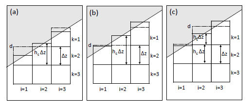
Synchronous coupling addresses these issues. The schematic above from (Jordan et al, 2018) gives the basic idea of how this is done. The ocean model discretises the ocean into boxes, or cells. In the MITgcm the top cell below the ice shelf (grey) can change its thickness. When the ice thins significantly the cells become too thick and the discrete approximation to the equations breaks down – but at this point the cell is split in two. In this manner, ocean computation is continuous and properties are conserved. Related developments have been made to allow the grounding line to retreat on-line (Goldberg et al, 2018). The movies below show three experiments with the coupled model where an ice shelf cavity is forced by downstream conditions with either a deep, mid-depth, or shallow thermocline. Melt rate along the evolving bottom surface of the ice shelf is plotted. Note that in the “hot” simulation, a piece of the ice shelf separates completely – an iceberg is formed! (More work would be required for this mass to have the proper dynamics of a large berg – but if you would like to take this on, get in touch with me!)

Relevant publications:

Jordan et al 2018
Goldberg et al 2018

Transient response to climate variability

Using coupled models, the question is often asked: what is the effect of a permanent change in ocean temperatures on ice sheets? However, there is mounting evidence that the largest signal of change in the Amundsen Sea is an interannual cycle, which dwarfs any prolonged trend. Ocean temperatures on the continental shelf are related to winds over this part of the southern ocean, and the strength of these winds is related to global-scale climate patterns, such as El Nino/ENSO. How does the frequency content of such climate forcing affect the response of the ice sheet, both in the short and the long term.

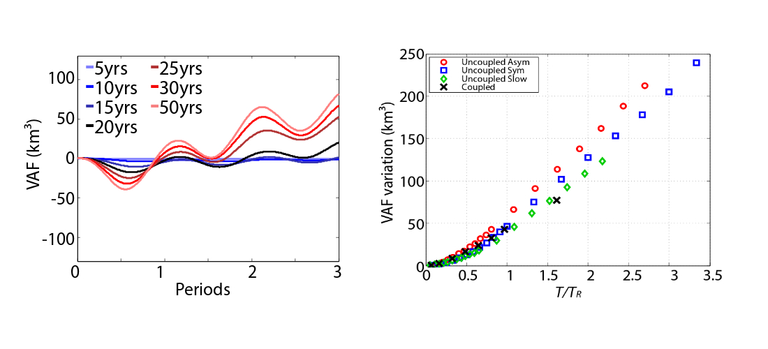
In (Snow et al (2017), the synchronously coupled model described above was applied to an idealised setup of a marine ice stream/shelf, the far-field ocean thermocline was oscillated at a range of frequencies, and the response in Volume Above Flotation (VAF) – the volume of an ice sheet that can contribute to sea level – was analysed. In the figure, the results over a number of periods is shown – clearly, there is a trend in sea level change even though the long-term average of ocean temperatures remains constant. In this case there is an increase in ice sheet volume but in general this will depend on specifics of bathymetry, topography, and the climate forcing. In the short term, the amplitude of response in VAF depends nonlinearly on the length of the period, such that a small change in frequency content of ENSO could lead to a large response in the amplitude of ice sheet change – potentially enough to trigger a marine instability.

Relevant publications:

Snow et al 2017